Transform and plot a spectrum

In this lesson you will normalise the peak of your film’s FTIR spectrum, then optionally plot the two curves. By the end you will have a new recorded result and a recipe linking it to the measured values, which stay unchanged. Allow about ten minutes.

The example picks up the sample and raw handle from Record your first measurement. Keep that session open, or rerun the earlier example first; the block below contains only the new work. Plotting needs matplotlib, installed separately in that environment, and you can skip that block entirely.

Write down the scientific choice

“Normalise this spectrum” sounds like a simple instruction, but it leaves several choices open. Which peak should count? Are you comparing signed values or magnitudes? What should the new maximum be? MTRL should not make those decisions on your behalf. Here you will write a small function that scales by the largest signed absorbance value and brings it to a chosen target.

The function checks that its maximum is finite and non-zero before dividing. That is a useful numerical safeguard, not proof that this is the right normalisation for your experiment. You remain responsible for the scientific choice.

Once you have the function, sample.transform handles the record-keeping. Give it the original handle and your callable. The params dictionary supplies the callable’s keyword arguments; name separately names the result you want MTRL to commit.

Normalise without losing the measured curve

Add the example below to the same session. It passes the recorded handle to your function and prints both peak heights, so you can see the new curve and the untouched original side by side.

Optional plotting dependency: matplotlib. NumPy calculates the values; matplotlib draws and displays the figure. The committed example needs only the base install; the plotting block below it needs matplotlib.

def normalise_peak(data, *, target=1.0):
    peak = float(data["absorbance"].max())
    if not np.isfinite(peak) or peak == 0.0:
        raise ValueError("absorbance has no finite, non-zero maximum")
    output = data.copy()
    output["absorbance"] *= target / peak
    return output


normalised = sample.transform(
    raw,
    normalise_peak,
    params={"target": 1.0},
    name="normalised",
)
print(f"normalised peak: {float(normalised.to_numpy()['absorbance'].max())}")
print(f"original peak: {round(float(raw.to_numpy()['absorbance'].max()), 4)}")

normalised peak: 1.0
original peak: 1.0075

The new curve reaches the target, while the measured peak keeps its original value. You now have both results, rather than one array whose earlier values you must remember.

Look at the curves, if you like

A figure is often the quickest way to see what a transformation did. If you want to draw one, install matplotlib into the same environment, for example with uv pip install --python .venv/bin/python matplotlib. Run this block after the example above, in the same session, so raw and normalised are still available:

import matplotlib.pyplot as plt

original = raw.to_numpy()
processed = normalised.to_numpy()

figure, axes = plt.subplots(figsize=(7.0, 4.0), layout="constrained")
axes.plot(
    original["wavenumber"], original["absorbance"],
    linewidth=1.8, label="Measured",
)
axes.plot(
    processed["wavenumber"], processed["absorbance"],
    linewidth=1.8, linestyle="--", label="Normalised",
)
axes.set_xlabel("Wavenumber / cm^-1")
axes.set_ylabel("Absorbance / a.u.")
axes.set_title("FTIR spectrum before and after peak normalisation")
axes.grid(alpha=0.25)
axes.legend(frameon=False)
plt.show()

Your figure looks like this one, drawn from the same data and code:

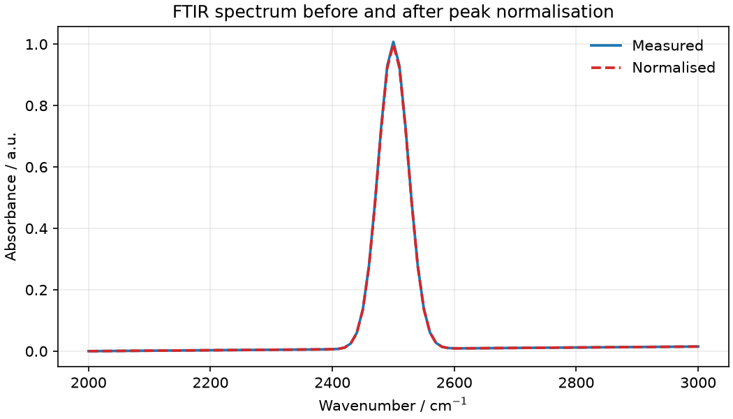
The solid measured curve keeps its original peak, while the dashed normalised copy reaches 1.0 exactly. The plot reads detached arrays; it does not change either record. You can choose colours, change a legend or add a visual offset in your plotting code without committing a scientific result. Use transform when the change is part of the analysis, not merely how you display it.

What just happened?

transform gave your function a detached, writable array and committed its output in one new revision. The result’s lineage records the exact input version and the effective parameters, including defaults. Later, when someone asks how you obtained the curve, that relationship is part of the record rather than something to reconstruct from a figure.

There is an important limit to that recipe. MTRL records your function’s name as custom provenance, but it does not store the executable code or make the function replayable. Keep your analysis code as well as your archive. The stored result can still be read without executing that code again.

This function keeps the same fields and preserves their declared units. The original record remains unchanged throughout.

Caution

MTRL does not establish the physical validity of a custom function. If you change fields or their physical meaning, declare the complete output units explicitly. Omitting units preserves declarations only under the facade’s documented field rules.

Tip

Peak normalisation is not a built-in operation. The registry guide, linked from the next lesson, explains reviewed, named operations and their replay contract.

Where next

You have been using handles without needing to unpack them. Look underneath a result explains what they name and shows how sample.core gives you access to the same history when a task outgrows the facade.